“Necessity is the mother of invention,” this proverb rings true when it comes to calculating grades and student titles for teachers, especially with large classes, multiple subjects, and the time-consuming and error-prone nature of manual calculations. So, how can you solve this problem? The secret lies in your “companion” – Microsoft Excel! This article will guide teachers on how to calculate student titles in Excel simply, efficiently, and quickly, helping you free up time to focus on teaching.
Grade Point Average (GPA) Calculation and Classification Formulas
Calculating GPA
The formula for calculating GPA in Excel is extremely simple. You just need to use the AVERAGE function to calculate the arithmetic mean of the grade columns. For example:
- =AVERAGE(B2:B10): Calculates the average grade for students in the Math grade column from row 2 to 10.
Student Classification Based on GPA
To classify students based on their GPA, you can use the IF function and corresponding classification conditions.
- =IF(AVERAGE(B2:B10)>=8, “Excellent”, IF(AVERAGE(B2:B10)>=6.5, “Good”, IF(AVERAGE(B2:B10)>=5, “Average”, “Weak”))): This formula will use the student’s GPA (calculated using the AVERAGE function) to provide the corresponding classification result: Excellent, Good, Average, Weak.
Creating a Student Title Table
Data Preparation
To create a student title table, you need a list of students, grade columns for each subject, and a GPA column.
Creating a Title Column
The next step is to create a title column. You can name this column “Title” or something similar.
Using the VLOOKUP Function
To automatically rank students based on their GPA, you can use the VLOOKUP function. The VLOOKUP function will search for a student’s GPA in a table and return the corresponding title.
- Create a GPA and Title Table: Create a separate table with two columns: GPA column and corresponding title column. For example:
| GPA Range | Title |
|---|---|
| 8.0 – 10.0 | Excellent |
| 6.5 – 7.9 | Good |
| 5.0 – 6.4 | Average |
| < 5.0 | Weak |
- Apply the VLOOKUP Function: Use the VLOOKUP function in the title column to search for the student’s GPA in the GPA table and return the corresponding title.
- =VLOOKUP(C2, $E$2:$F$5, 2, FALSE): This formula will search for the GPA of the student in cell C2 in the GPA and title table from cells E2 to F5, return the value in the 2nd column (title column), and only perform exact matches (FALSE).
Important Notes When Using Excel
Choose the Appropriate Method
Remember that there is no one-size-fits-all method. Depending on your needs and the complexity of the grade sheet, you can choose the most suitable method.
Thoroughly Check
After creating the spreadsheet, check it thoroughly to ensure the accuracy of the results.
Regular Updates
To ensure the spreadsheet is always up-to-date, regularly update new data and double-check the formulas.
Advice from Experts
According to Mr. Nguyen Van A, author of the book “Information Technology in Education,” using Excel to calculate student titles is an effective method that saves time and improves the efficiency of teachers’ work. However, he also emphasizes that the use of technology needs to be accompanied by careful checking to ensure the accuracy of the results.
An Excel Story
This story can be created according to your request to illustrate the effective use of Excel for calculating student titles. Imagine a young teacher, fresh out of graduation, facing the task of grading and calculating titles for a large class. Manual grading makes the teacher feel tired and prone to errors. The teacher is accidentally introduced to using Excel by a colleague. Thanks to this, the teacher solved the problem of grades and titles quickly and efficiently, and spent more time teaching.
Conclusion
Calculating student titles in Excel is no longer a difficult task. With the detailed instructions above, hopefully, teachers can easily apply them and improve their work efficiency. Try applying it now, and you will see surprising results!
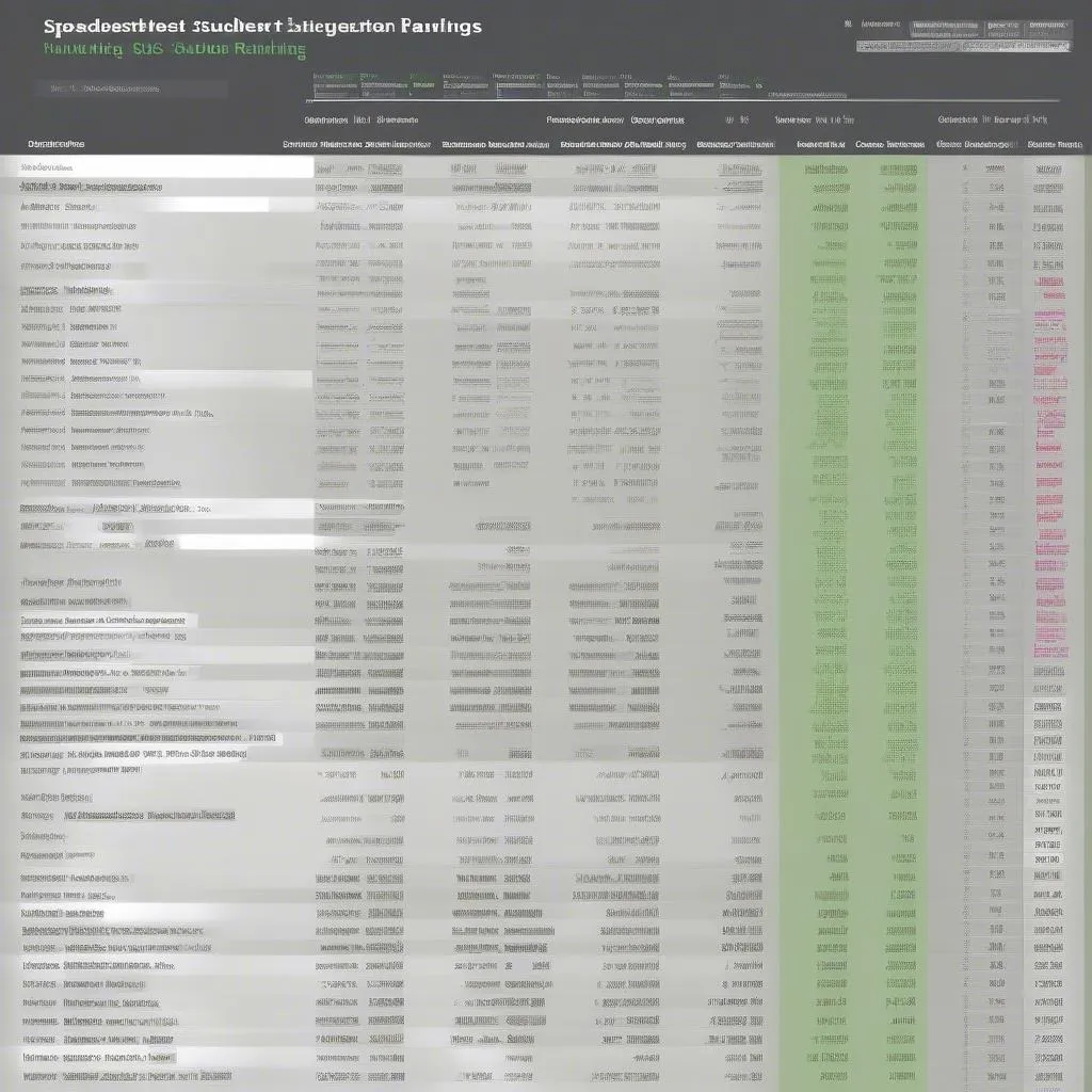
 Student grade sheet and titles